Probes & Grounding
Why Your Ground Lead Is Lying to You
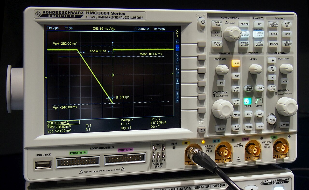
You are chasing a glitch on the finger-driver board of a robot hand: a clean 3.3 V step out of the gate driver that should switch a motor FET. You clip the scope probe tip to the gate, clip its little alligator ground to the nearest screw you can reach, and the screen erupts. A vicious overshoot, a fat ring that takes a dozen wiggles to die, a waveform uglier than anything the circuit could possibly be making. You did not measure the bug. You built one with your own probe.
A probe is not a window onto the circuit. It is another circuit you just soldered in.
Every measurement adds the instrument to the thing being measured, and a scope probe is no exception: it brings its own resistance, its own capacitance, and, through that innocent-looking ground lead, its own inductance and its own path to earth. Getting an honest trace is mostly about understanding what the probe adds and connecting it so that those additions stay small. The whole craft rests on one ordering rule: respect the ground first, then the tip, because the ground return, not the pointy end, is where almost every probing lie is born.
By the end, you can
- Explain why a single-ended passive probe measures against earth-referenced ground, and why its ground clip can short a live node to earth
- Calculate the minimum scope and probe bandwidth from a signal's rise time using the 0.35 rule
- Predict the ringing on a fast edge from the ground-lead inductance and probe capacitance, and choose the short spring to fix it
- Choose between a 1x and a 10x passive probe by reasoning about how much each one loads the circuit
Intuition first
Think of the scope probe as a stethoscope, but a strange one: it has to touch the patient at two points, not one. There is the tip, which presses on the node you care about, and there is the ground lead, which presses somewhere the scope can agree is “zero.” A doctor’s stethoscope only listens. This one also connects the patient to the wall, because the far end of that ground lead runs all the way back through the scope chassis to the third pin of the mains plug, to earth.
That second contact point is where beginners get burned twice. The first burn is electrical and literal: clip the ground to a node that is not actually at ground potential and you have just wired that node to earth through the scope. The second burn is subtle and shows up on the screen: the ground lead is a loop of wire, and a loop of wire is an inductor. Pair that inductor with the small capacitance the probe presents and you have built a tuned circuit that rings like a bell every time the signal takes a fast step. The cure for both is the same instinct: keep the ground connection short, deliberate, and honest, and only then worry about the tip.
The ground clip shorts the node to earth
A standard passive probe is single-ended: it reports the voltage of one node measured against the scope’s own ground, and that ground is bonded to mains earth through the power cord. So the reading is always “tip minus earth,” never “tip minus some arbitrary node of your choosing.”
Now picture what the ground clip physically does. It is a low-resistance wire from the probed board straight to earth. Clip it to a node that genuinely sits at 0 V and nothing happens: you have connected earth to earth. Clip it to a node that is not at 0 V, say a switch node swinging between 0 V and the motor rail, and you have bolted that node to earth through a few tens of milliohms of alligator clip. The node can no longer move. Either the supply slams current into the short and something lets go, or, on a mains-referenced supply, fault current flows through you and the bench. The scope did not measure the node. It clamped it.
The diagram shows the other half of the story, the part that bites even when your ground clip is on a perfectly good ground. The long ground lead and the probe tip do not just carry signal. They enclose area, and that area is the body of an inductor in series with a capacitor. That is the loop we have to tame next.

The ground lead rings because it is an L-C tank
Here is the part of probing that feels like black magic until you name it. The ground lead is a wire, and any wire has inductance roughly proportional to the area of the loop it forms. A typical 10-15 cm alligator-clip lead is around 50-150 nH. The probe tip, meanwhile, presents a small capacitance to ground, on the order of 10-15 pF for a 10x probe. An inductor and a capacitor in a loop make a resonant tank, and a tank has a natural frequency
where is the ground-lead inductance and is the probe-plus-input capacitance. Plug in and and you get
Nothing rings until something kicks the tank, and a fast signal edge is exactly that kick. A step contains energy at frequencies far above its repetition rate (more on that in the Go Deeper), and when that energy lands on a resonance the tank answers with a damped sinusoid: overshoot, then a decaying ring at . The faster your edge, the harder the kick, and the uglier the ring. This is why the same probe looks perfect on a slow 1 kHz square wave and disgraceful on a 5 ns gate edge. The circuit did not change. The probe’s tank just got excited.
The fix is not a better scope. It is a shorter ground. Inductance falls with loop area, so swapping the long flying lead for the short ground spring (the little sprung collar that lets the barrel touch ground millimeters from the tip) drops from tens of nanohenries to a few. Push down by 10x and climbs by a factor of about three, often clear past the scope’s bandwidth where it can do no harm, and the overshoot shrinks with it. The long lead is a convenience for slow signals. For anything fast, it is the single biggest source of measurement error you control with your own hands.
Bandwidth: pick the scope before you plug in
Inductive ringing is the error you make at the bench. Bandwidth is the error you make at the catalog, by reaching for an instrument too slow to see the edge in the first place. The governing relationship between an edge’s rise time (the 10% to 90% transition) and the bandwidth needed to reproduce it is
The 0.35 falls straight out of a single-pole low-pass response, the simplest model of a band-limited channel: such a system’s own 10% to 90% rise time is , and that number is fixed by the natural log arithmetic of an exponential settling toward its final value. So a 1 ns edge demands at least just to be seen, and “seen” here means barely, with the edge already softened.
Barely is not good enough, because bandwidths add in quadrature, not linearly. Feed a 350 MHz signal through a 350 MHz scope and the displayed edge is noticeably slower than the real one. The working rule is to aim for the scope (and probe) bandwidth at roughly five times the signal’s knee frequency, where the knee is the frequency content implied by the rise time, . Five times the knee buys you flat response through the part of the spectrum that defines the edge’s shape, so the trace you read is the edge the circuit actually makes, not a filtered ghost of it. Under-buy bandwidth and every edge looks slower and softer than reality, which can fool you into thinking a perfectly snappy driver is sluggish.
You clip a passive probe's ground alligator to a metal heatsink tab that is electrically tied to a high-side switch node swinging 0 to 24 V. What happens?
-
A single-ended probe measures against earth, not against whatever you clipped to. The clip does not float to the node, it drags the node to earth.
-
Correct. The ground clip is hard-wired to mains earth through the scope. Clipping it to a non-ground node bolts that node to earth, and the supply (or the switch) dumps current into the short.
-
The 10x divider sits in the tip path. The ground lead is a near-zero-ohm wire to earth and offers no protection at all.
-
There is no clean attenuation here, there is a short. The node cannot swing because it is pinned to earth.
See it / Try it
The simulator below builds the probe’s ground-lead tank and lets you excite it with a fast edge. Start with the default long lead, watch the overshoot and the decaying ring, then tick the short ground spring box and watch the inductance, the ring frequency, and the overshoot all respond.
- Inductance L
- 50 nH
- Ringing f
- 205 MHz
- First overshoot
- 38%
Drag the ground-lead length up and the inductance climbs, the ring frequency drops into the band the scope can show, and the overshoot grows: that is the ugly fat ring from the Hook, reproduced on demand. Now check the short-spring box. The inductance collapses to a few nanohenries, leaps upward (often above where it can do visible harm), and the overshoot shrinks toward nothing. You did not touch the circuit under test once. Every change on screen came from how you connected the ground. That is the whole lesson in one toggle: the probe’s ground return, not the signal, is writing most of what you see on a fast edge.
A clean step out of a gate driver shows 40% overshoot and a long 200 MHz ring on your scope. Swapping nothing but the long ground lead for the short ground spring mostly cures it. Why?
-
The spring changes the ground return, not the divider ratio. Attenuation is unchanged.
-
Correct. Inductance scales with loop area. The short spring shrinks the loop, drops L from tens of nH to a few, pushes f_ring up (often past the scope's bandwidth), and damps the overshoot.
-
The spring removes inductance, it does not add capacitance. Adding C would lower the ring frequency, not cure the ring.
-
Earth bonding is set by the power cord and is irrelevant to the L-C ring at the probe tip.
Lab
On the bench, prove the tank to yourself in three minutes. Probe the scope’s own 1 kHz calibrator and compensate the 10x probe until the square corners are crisp. Then find any fast edge you have (a GPIO toggle, a PWM channel from Lesson #9, a logic clock) and capture it twice without changing anything else: once with the long alligator ground lead, once with the short ground spring touching ground right next to the tip. Photograph both. Measure the overshoot percentage and the ring period each time, and turn the ring period into a frequency. You will see the ring frequency jump and the overshoot collapse on the short ground, exactly as the simulator promised. Finally, read the fastest edge’s 10% to 90% rise time off the screen and check it against your scope’s rating: if comes out near or above your scope’s bandwidth, the edge you are looking at is being softened by the instrument and you need a faster scope to trust it.
Why a sharp edge needs so much bandwidth, and where 0.35 actually comes from
A step edge looks like one event in time, but in frequency it is a whole comb of harmonics. The faster the transition, the higher up that comb the meaningful energy reaches. A useful shorthand is the knee frequency, the point below which a digital edge’s spectrum carries the energy that defines its shape:
Reproduce the channel flat to a few times and the edge keeps its shape; cut it off near the knee and the corners round over. That is why “5x the knee” is the buying rule, not “1x the knee.”
The famous 0.35 is the rise time of the simplest band-limited channel, a single-pole RC low pass. Feed it a step and the output is . Solve for the 10% and 90% crossing times and subtract:
so
Real scopes are closer to a Gaussian channel, for which the constant is about 0.34, near enough that 0.35 is the universal rule of thumb. And because cascaded stages add in quadrature, the scope-plus-probe system rise time is , which is why a probe far faster than the scope barely slows the system while a probe slower than the scope wrecks it.
One reconciliation with the authoritative bench rule: the grounding text frames it as scope/probe for the fastest edge you must capture, then nudges you to roughly 5x the knee for honesty. The Wikipedia derivation gives the same 0.35 as a property of the channel itself (its own rise time), measured the other way round. They are two faces of one identity, : read left-to-right it sizes the instrument, read right-to-left it tells you how much the instrument will soften an edge.
Grounded in Wikipedia: “Oscilloscope”, “Test probe”, “Ground loop (electricity)”, “Rise time” (CC BY-SA).
Key takeaways
- A passive single-ended probe measures tip minus earth; its ground clip is hard-wired to mains earth, so clipping it to a non-ground node shorts that node to earth.
- The ground lead's inductance plus the probe's capacitance form an L-C tank that rings on fast edges at $f_{\text{ring}} = 1/(2\pi\sqrt{LC})$.
- Use the short ground spring, not the long flying lead: less loop area means less inductance, a higher ring frequency, and smaller overshoot.
- Bandwidth rule: scope and probe $\text{BW} \ge 0.35 / t_{\text{rise}}$ for the fastest edge, and aim for about 5x the knee frequency for an honest trace.
- A 10x passive probe loads the circuit about 10x less than a 1x probe; reach for 10x by default and only drop to 1x for tiny signals.
The fastest edge you need to capture on the finger-driver board has a rise time of . What is the minimum scope bandwidth, and what bandwidth would you actually buy for an honest trace?
Show worked solution
Minimum bandwidth from the 0.35 rule:
That only lets you see the edge, already softened. For an honest trace, target about five times the knee frequency. The knee is , so aim for roughly . In practice you would reach for the next standard scope above that, say a 1.5 GHz instrument, and make sure the probe is at least as fast.
Your probe’s tip capacitance plus scope input is . With the long alligator lead the ground inductance is ; with the short spring it is . Find the ring frequency in each case and explain what the change does to the trace.
Show worked solution
Use .
Long lead:
Short spring:
Cutting by 30x raises by about times, from 133 MHz to roughly 727 MHz. On a mid-range scope the 133 MHz ring sits squarely in the displayed band and smears every fast edge; the 727 MHz ring is often above the scope’s bandwidth entirely, so it is filtered out and the displayed overshoot shrinks toward nothing. Same circuit, honest trace, just by shortening the ground.
You are probing a high-impedance node: a resistor feeding a sensor input, carrying a 1 MHz signal. Compare a 1x probe (load about in parallel with ) with a 10x probe (about in parallel with ). Which loads the node less at 1 MHz, and by how much does the capacitance matter?
Show worked solution
At 1 MHz the resistive part barely matters next to the source’s , so the loading is dominated by the probe capacitance, whose reactance is .
1x probe, :
10x probe, :
The 1x probe presents only about to ground at 1 MHz, which is a brutal load next to a source: it would slug the node hard and roll off the signal. The 10x probe presents roughly , about 8x lighter, and its DC resistance is also 10x kinder. On a high-impedance node the 10x probe is the only honest choice; the 1x probe loads the circuit roughly an order of magnitude harder and would falsify the very measurement you came to make.
The probe was never a window. It is a guest you invite into the circuit, and like any guest it changes the room a little just by standing in it. Honor the ground return before the tip, keep the loop tight, size the bandwidth to the edge, and the guest stays quiet enough to trust. Forget, and the lie you read on the screen is one you wrote yourself, in a loop of wire no longer than your thumb.